TL;DR
We built the loop a customer would actually run: labelled rows arrive over time, and every time a batch lands, vega refits one small head per question on a frozen reader, recalibrates on rows the heads never saw, writes a new versioned calibration file and serves it. Nothing is trained. Then we scored it after every batch against TypeSafe's Jev 1.14, live, on the same held-out rows.
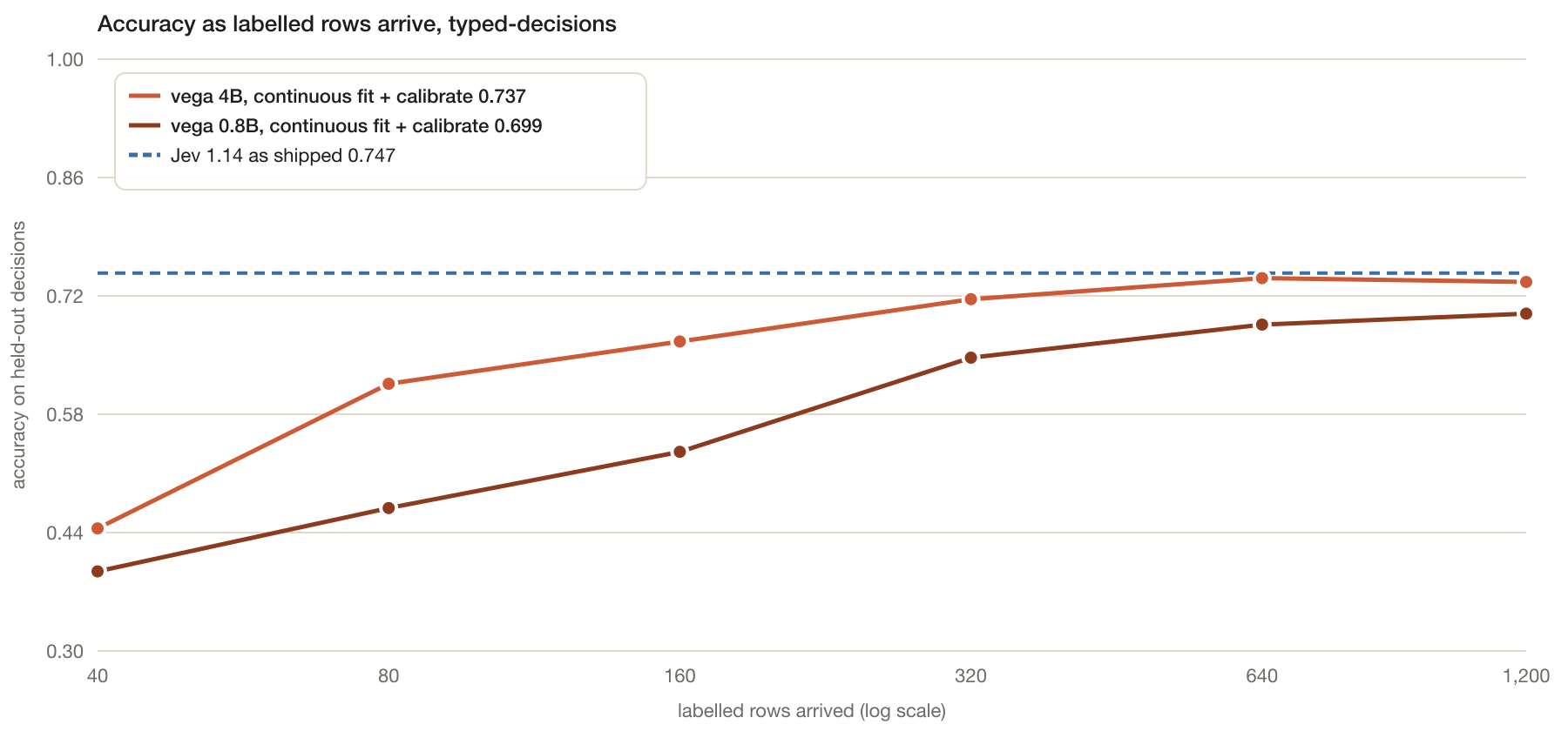
- On a bespoke workflow benchmark (four workflows, five typed questions per case, 1,200 rows arriving), vega 4B went from 44.5% cold to 73.7%, which is level with Jev as shipped at 74.7%, with a third less calibration error and a review band Jev does not have.
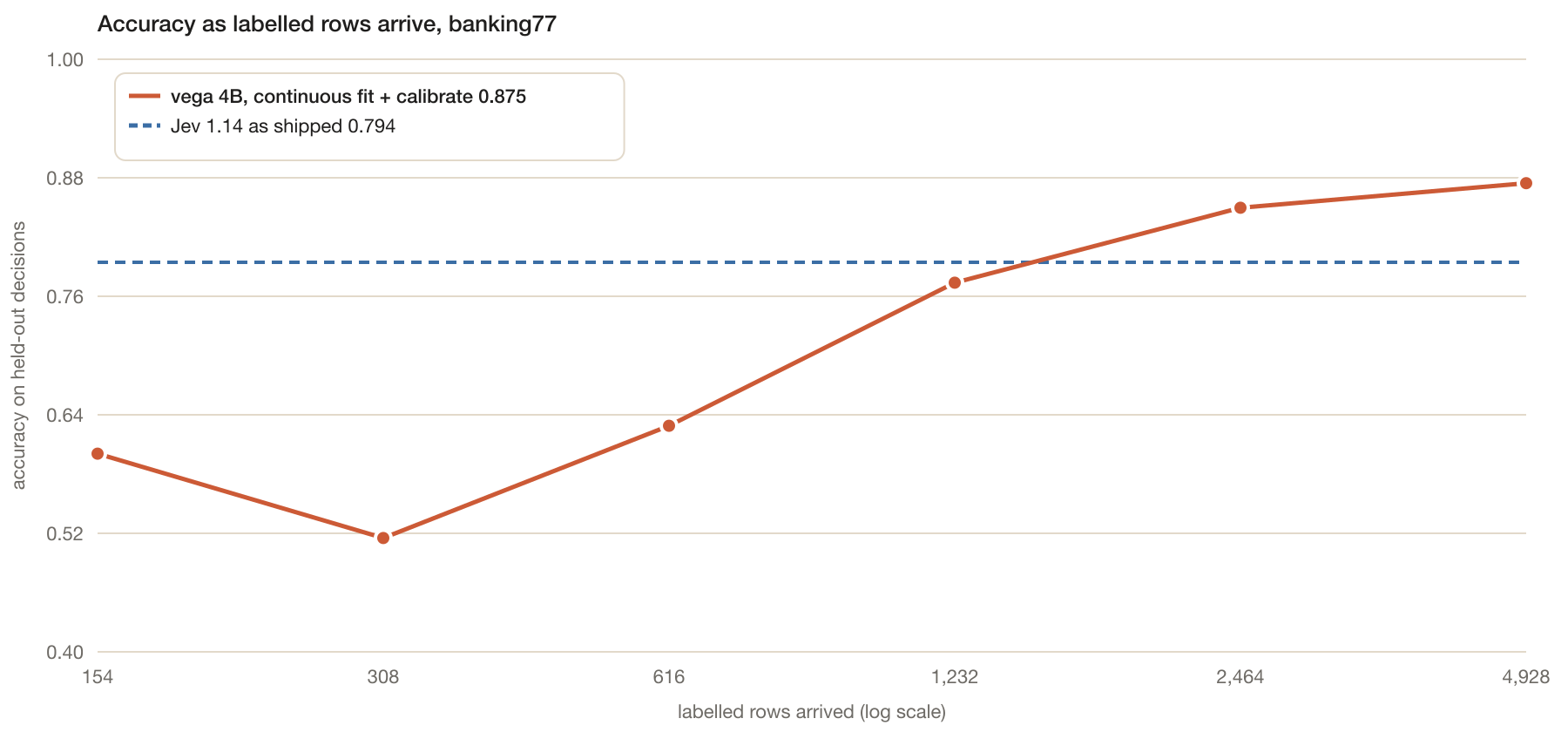
- On a 77-way customer intent stream (4,928 rows arriving), vega 4B went from 60.1% cold to 87.5%, eight points past Jev as shipped at 79.4%, and by the end it was handling 92.5% of the traffic automatically at a measured 91.5% precision.
- The ablation that matters for anyone building this: calibrate on the rows you fitted on and the file tells you to automate 100% of the traffic at ECE 0.26. Calibrate on held rows and it is ECE 0.03 with a band whose precision holds. Same heads, same accuracy, opposite routing decisions.
- Every Jev call in the whole study cost under a dollar at the published price. Cost is not the argument. Calibration, the band, a versioned file per batch, and rows that never leave your network are the argument.
Every table in this post, the per-round tables, the per-type breakdowns, the calibration tables at every confidence floor and the latency and cost lines, is in the full technical report (PDF), and the run itself is a public Kaggle notebook.
Why fine-tuning is the wrong tool for this job
Every decision model on the market learns your labels the same way: run a gradient through the language model until it agrees with you. Jev is a fine-tune. Prism is a LoRA on a 105B model. Our own laya checkpoints are fine-tunes too, and that is the better version of the idea, with reinforcement learning against a proper scoring rule. It is still the same idea.
Fine-tuning is a fine tool when the task is fixed, the data is all there, and someone pays for the GPU once. It is the wrong tool for a customer whose data arrives every day, for four reasons we have hit ourselves.
- It is a training job per batch. Hours on a GPU, a learning-rate schedule, early stopping that can cut the run short. Our E4B fine-tune stopped itself at 2.2 of 9.5 hours once, and nobody noticed until the numbers came back wrong. You cannot run that unattended on Tuesday's rows and again on Wednesday's.
- It always produces a model. Fine-tuning never says "these 40 rows taught me nothing". You find that out from a separate evaluation, if you built one.
- One question moves the others. Weights are shared. Fine-tune for the urgency question and the routing question shifts underneath it, so every batch means retraining and re-evaluating every question.
- You cannot roll it back or audit it. A fine-tune is a new model per customer per version. The thing a bank's auditor asks for, "which version made this decision in March and what did it know", is a hard question to answer with a pile of checkpoints.
And one honest number. Fine-tuning has the higher ceiling when you have the data and the budget: our laya fine-tune on the same workflow benchmark reached 76.6%, above Jev and above the 4B fit. We are not claiming the loop beats a dedicated fine-tune on a fixed task. We are claiming it is the only one of the two you can leave running.
What fit and calibrate do instead
The reader is a frozen language model, 0.8B or 4B parameters here. It never sees a gradient. It turns a state and a question into a feature vector , and because the reader is frozen, that vector can be cached: a refit reads only the rows that are new since the last one.
Fit is one linear head per question. Standardise the features, project onto the top principal directions, then a multinomial logistic fit with an penalty:
That is convex, a few hundred steps on a tiny matrix, seconds on a CPU. The head is cross-validated and it is allowed to lose: it is kept only if its cross-validated accuracy beats chance, and it is served only if it also beats the frozen engine's own accuracy on the same rows. A head that learned nothing is discarded, and the loop tells you so.
Calibrate runs on rows the head never saw, and fits three numbers per question. A temperature that rescales the probabilities, found by minimising negative log-likelihood. A conformal threshold: with scores on the held rows, is the -th smallest, and the set of options with contains the right answer at least of the time on data like these rows. And a review line : the widest band of confidences above whose precision holds at the target, using Wilson's lower bound rather than the observed hit rate,
so that twelve for twelve on twelve rows does not count as a 100% precision band. If no line can hold the target, the band says so and routes everything to review. All of it is written to one JSON file stamped with the checksum of everything that changes an answer. That file is the deployment: every decision carries its version.
The deeper write-up of each step, with the theorems, is in Fit and calibrate, not fine-tune. This post is what happens when you run it as a loop against a hosted competitor.
The experiment
Two public streams, each played as arrivals. At each round, about a quarter of the arrived rows are held for calibration (chosen by a hash of the row id, so a row that calibrated at round three still calibrates at round four) and the rest fit the heads. After every round the same held-out set is scored. Jev 1.14 is called live on the same held-out rows, pinned to jev-1.14.0, with the dataset's own state and questions as the request body.
| stream | what it looks like in a business | arrivals | held out |
|---|---|---|---|
| typed-decisions | support threads, vendor invoices, security alerts, agent traces; five typed questions per record | 1,200 cases | 400 cases, 2,000 decisions |
| banking77 | one customer message, which of 77 banking intents | 4,928 rows | 924 rows, stratified |
Jev has no fit and no calibration endpoint. What a customer gets is the cold model, so that is the headline comparison. We also measured the two things a customer could do with the same labelled rows: write them into Jev's criteria as examples, which is the only tuning surface its API has, and put Jev's answers behind our own calibration layer. Those come later in the post.
Stream one: a bespoke workflow taxonomy
| arm | rows used | accuracy | ECE | auto at 90% precision | precision in band |
|---|---|---|---|---|---|
| Jev 1.14 as shipped | 0 | 0.747 | 0.047 | no band | n/a |
| vega 0.8B cold | 0 | 0.394 | 0.208 | no band | n/a |
| vega 0.8B, continuous | 1,200 | 0.699 | 0.040 | 14.6% | 0.935 |
| vega 4B cold | 0 | 0.445 | 0.170 | no band | n/a |
| vega 4B, continuous | 320 | 0.716 | 0.051 | 7.8% | 0.852 |
| vega 4B, continuous | 640 | 0.741 | 0.035 | 10.5% | 0.972 |
| vega 4B, continuous | 1,200 | 0.737 | 0.031 | 15.0% | 0.943 |
Read it as a customer would. Out of the box, Jev gets three in four decisions right. vega with no labels gets fewer than half. After the customer's own 1,200 rows have flowed through the loop, the 4B reader gets three in four as well. The gap between 0.737 and 0.747 is inside one standard error for 2,000 decisions, so we call it level and we do not call it a win.
Where it is not level is the number next to the answer. vega's calibration error is a third lower than Jev's, and vega can say which 15% of decisions are safe to automate at 94% precision. Jev returns probabilities but no band, so it cannot say that at all.
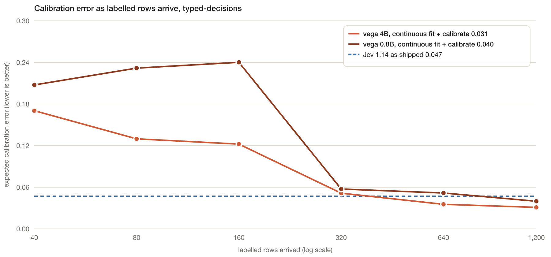
One more thing the curve says. The returns halve with every doubling of rows: 320 to 640 bought four points, 640 to 1,200 bought none. The thing that moved this stream from 0.699 to parity was the reader, 0.8B to 4B, not more rows. On a frozen reader, labels can only sharpen what the features already separate.
Stream two: 77 intents, thousands of messages
| arm | rows used | accuracy | ECE | auto at 90% precision | precision in band |
|---|---|---|---|---|---|
| Jev 1.14 as shipped | 0 | 0.794 | 0.078 | no band | n/a |
| vega 4B cold | 0 | 0.601 | 0.251 | no band | n/a |
| vega 4B, continuous | 616 | 0.629 | 0.052 | 2.6% | 1.000 |
| vega 4B, continuous | 1,232 | 0.774 | 0.046 | 61.0% | 0.922 |
| vega 4B, continuous | 2,464 | 0.850 | 0.038 | 86.7% | 0.906 |
| vega 4B, continuous | 4,928 | 0.875 | 0.028 | 92.5% | 0.915 |
This is the stream the loop is for. Short messages, many categories, and a customer who has thousands of them. The band opens as the calibration rows accumulate: 2.6% automated at 616 rows, 61% at 1,232, 92.5% at 4,928, and the precision inside the band stays at or above the 90% it was asked for every time. The dip at 308 rows is real: four rows per intent is enough to pass cross-validation and not enough to beat the engine on every intent, and the harness served the head anyway because on average it won. By 616 rows it had recovered.
What that means on a desk. Take a bank that gets 100,000 messages a day. With this file, 92,500 are answered automatically and about 7,900 of those are wrong, which is the 91.5% precision; 7,500 go to a person with a reason attached. With Jev as shipped you get 79,400 right and 20,600 wrong, and no instrument to pick the subset you would trust, because there is no band. The accuracy gap is eight points. The operational gap is that one of the two can be put on autopilot and the other cannot.
The ablation, and what it means for the business
Every arm below starts from the same arrived rows at the final round, 4B reader, both streams. This is the table to show anyone who wants to build a self-improving loop, because it contains the way to build it wrong.
| arm | typed-decisions acc | ECE | auto | banking77 acc | ECE | auto |
|---|---|---|---|---|---|---|
| engine cold, nothing fitted | 0.445 | 0.170 | n/a | 0.601 | 0.251 | n/a |
| engine + calibrate, no heads | 0.445 | 0.053 | 4.2% | 0.601 | 0.091 | 14.3% |
| heads, no calibrate | 0.737 | 0.124 | n/a | 0.875 | 0.243 | n/a |
| heads + calibrate on the fitting rows | 0.737 | 0.258 | 100% | 0.875 | 0.051 | 100% |
| heads + calibrate on held rows (the product) | 0.737 | 0.031 | 15.0% | 0.875 | 0.028 | 92.5% |
| heads on every row, no calibration split | 0.753 | 0.117 | n/a | 0.885 | 0.245 | n/a |
Four things fall out of it.
- The heads carry the accuracy; the calibration carries the trust. Heads alone reach the same accuracy as the product and their calibration error is four to eight times worse. Calibration alone fixes the error and changes no answers. You need both, and they are separable, which is why the file can be refitted without touching the heads.
- Calibrating on the fitting rows is the trap. On typed-decisions it reports ECE 0.258 and routes 100% of decisions to automatic. The head has memorised those rows, so its confidence on them is a story, and the temperature and the band believe the story. Any loop that fits and calibrates on the same buffer will ship this file and call it safe. Hold a quarter of the rows out. Always.
- The band costs about one point of accuracy. Fitting on every arrived row with nothing held out buys 0.753 and 0.885. The quarter you hold for calibration is the price of knowing which answers to trust, and it is a price worth paying on any stream where a wrong automatic decision costs more than a reviewed one.
- Calibration does not need the heads. The cold engine behind a calibration file goes from ECE 0.17 to 0.05 with no accuracy change. That is the first thing a new customer gets, before they have enough labels for a head.
What Jev can do with the same rows
Its API has no fitting surface, so the labelled rows can only go into the request. We wrote up to two state excerpts per option into each option's criteria (the tuned arm), and separately we fitted our own temperature, conformal threshold and band on Jev's answers to the calibration rows (the layer arm).
| arm | typed-decisions acc | ECE | auto | banking77 acc | ECE | auto |
|---|---|---|---|---|---|---|
| Jev as shipped | 0.747 | 0.047 | no band | 0.794 | 0.078 | no band |
| Jev + examples in criteria, 80 / 308 rows | 0.752 | 0.034 | no band | 0.857 | 0.042 | no band |
| Jev + examples in criteria, all rows | 0.746 | 0.026 | no band | 0.857 | 0.042 | no band |
| Jev + our calibration layer | 0.746 | 0.044 | 32.1% at 0.946 | 0.794 | 0.068 | 64.9% at 0.940 |
| vega 4B, continuous (for reference) | 0.737 | 0.031 | 15.0% at 0.943 | 0.875 | 0.028 | 92.5% at 0.915 |
Examples in the prompt help Jev on the intent stream, six points, and stop helping after the first few hundred rows; on the workflow benchmark they do nothing. They also multiply the tokens per call by five, forever. The layer arm is the one we find interesting: our calibration file works on someone else's model. Jev behind it gets a band it never had, 65% of banking traffic automated at 94% precision. If you already pay for a hosted decision model, this is the part you can add without changing anything else.
Cost and time, measured
| item | measured |
|---|---|
| Jev, all arms, both streams, 4,673 live calls | $0.65 at the published $0.042 per million input tokens |
| Jev per million decisions at this benchmark's token counts | about $8 |
| Jev request latency, median, from Kaggle | 85 to 97 ms |
| vega 4B refit at 1,200 arrived rows on one T4 | 20 minutes, almost all the engine cross-check |
| vega 4B, whole study on two T4s, both streams in parallel | 2 h 40 min |
| vega 0.8B feature read on an Apple M5 | 65 ms, cached after the first read |
So at benchmark scale cost is a rounding error on both sides, and we are not going to pretend otherwise. The refit time is worth a note: reading new rows is proportional to the arrival rate, but the engine cross-check that decides whether a head is worth serving reads every fitted row once. That is the one cost in the loop that grows with history, and it is the next thing to cache.
Where this leaves a buyer
If you have a bespoke workflow with a few hundred to a thousand labelled records, a frozen 4B reader with the loop matches a hosted decision model on accuracy, beats it on calibration, and is the only one of the two that tells you what to automate. If you have a stream of short messages with many categories and thousands of labels, the loop passes the hosted model and keeps going. In both cases the rows never leave your network, there is no meter, and every decision names the calibration version that made it.
What we are not saying: that the loop beats Jev on the workflow benchmark, because it does not, and that more rows would fix that, because the curve says they would not. The levers there are the reader, the 27B being the next one up, and the head itself. We will publish those runs when we have them, on the same held-out rows, with the same cached Jev answers, so the comparison stays honest.
Run the loop yourself
The loop is three calls in the public package. Everything the harness added on top was the arrivals, the hold-out by id, and the scoring.
pip install -U vegaml

import vegaml
from vegaml.calibrate import calibrate

V = vegaml.load("4b")                        # or vegaml.load() for the 0.8B

def held(row_id):                            # about a quarter of rows, by id, never by arrival order
    import hashlib
    return int(hashlib.sha1(row_id.encode()).hexdigest(), 16) % 4 == 3

def refit(arrived, questions, version):
    fit_rows = [(s, labels) for rid, s, labels in arrived if not held(rid)]
    cal_rows = [(s, labels) for rid, s, labels in arrived if held(rid)]
    report = V.fit(fit_rows, questions, folds=5)                # heads; each one allowed to lose
    cal = calibrate(V, cal_rows, questions, alpha=0.1,          # temperature, conformal threshold,
                    target_precision=0.90)                      # review band at 90% precision
    cal.save(f"calibration_{version}.json")                     # stamped with its checksum
    return report, cal

# every batch: arrived grows, refit runs, the new file serves
out = cal.apply(V.decide(state, questions))                     # probs, prediction_set, abstain, route
The full run is a public Kaggle notebook: kaggle.com/code/nandakishorconvai/vega-fit. Two T4s, typed-decisions on one GPU and banking77 on the other, the Jev key in a secret named JEV_API, and it writes the same results.json and per-round calibration files the report was built from. The datasets are LocalLLaMA/typed-decisions and PolyAI/banking77, so every number above can be checked line by line.